BPLG

The Butterfly Processing Library for GPUs (BPLG) is a high performance library for CUDA GPUs. It can be used to process algorithms that can be expressed through a butterfly structure. BPLG is very modular and was designed with simplicity and flexibility in mind. It is based on a series of basic functions or building blocks, which when combined properly, create the different algorithms.

The BPLG library supports several signal processing algorithms: the complex FFT, the real FFT, the DCT and the Hartley transform. To demonstrate its applicability, it was extended to also support other problems, like the resolution of tridiagonal systems. The full source code is provided, so it can be adapted to other problems or customized for the desired applications.

Following we summarize the performance the different transforms supported by the library executed on several GPU architectures. For a more detailed comparison including other well-known libraries, please check the publications in the documentation section.

The tests were evaluated in single precision using problem sizes in the range N = { 4, ... , 4096 } . Batch execution is used to process 2²⁴ / N different problems, therefore, as the input signal increases the number of batch executions decreases. All the data resides on the GPU memory at the beginning of each test, so there are no data transfers to CPU during the benchmarks.

Three different GPUs with different architectures were used in the tests:

•   GeForce Titan		Kepler architecture		reference clocks
•   GeForce 580		Fermi architecture		reference clocks
•   GeForce 750 TI		Maxwell architecture		Palit StormX Dual (1.2 GHz core, 6.0 GHz memory)

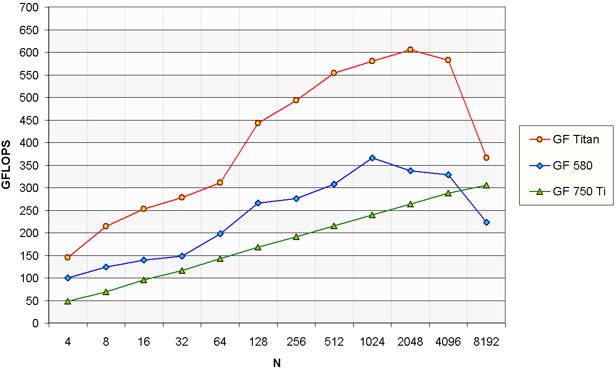
Complex FFT

The FFT (Fast Fourier Transform) is used in many real-world signal processing applications. For instance, image and video processing, pattern recognition or large number manipulation. The performance of the complex FFT is expressed in GFLOPS through the commonly used expression:

GFLOPS = 5N · log₂ ( N ) · b · 10^-9 / t

where N is the size of the input, b is the total number of signals processed and t is the time in seconds.

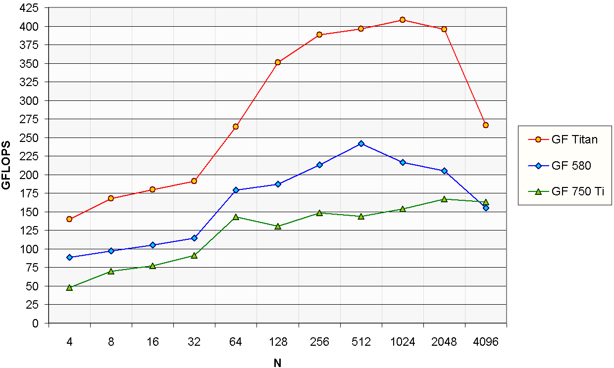
Real FFT

In some domains, like audio processing, the input signal is known to be purely real. Thus, taking advantage of this property, it is possible to perform an optimized version of the FFT with fewer operations and less memory bandwidth. A expression similar to the previous one can be used for the real FFT:

GFLOPS = 2.5N · log₂ ( N ) · b · 10^-9 / t

The change in the first coefficient is given by the reduction on the number of operations, which is approximately halved due to using real arithmetic instead of complex arithmetic.

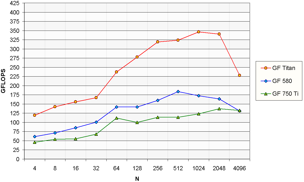
Hartley Transform

The Hartley transform also has a real input, but in contrast to the real FFT, its output is also real. Due to its simpler computation, it is used in some embedded and low power devices. As far as we know there is no standardized expression for the Hartley transform, therefore to offer a similar measurement we will use the same formula as the real FFT.

Discrete Cosine Transform

The DCT is widely used in lossy data compression due to its energy compaction properties. This transform is also designed to work on purely real data. Like in the case of the Hartley transform, as far as we know there is no standardized expression for the DCT, thus we will use the same expression as in the real FFT.

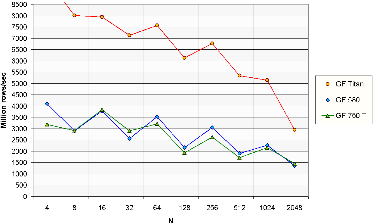
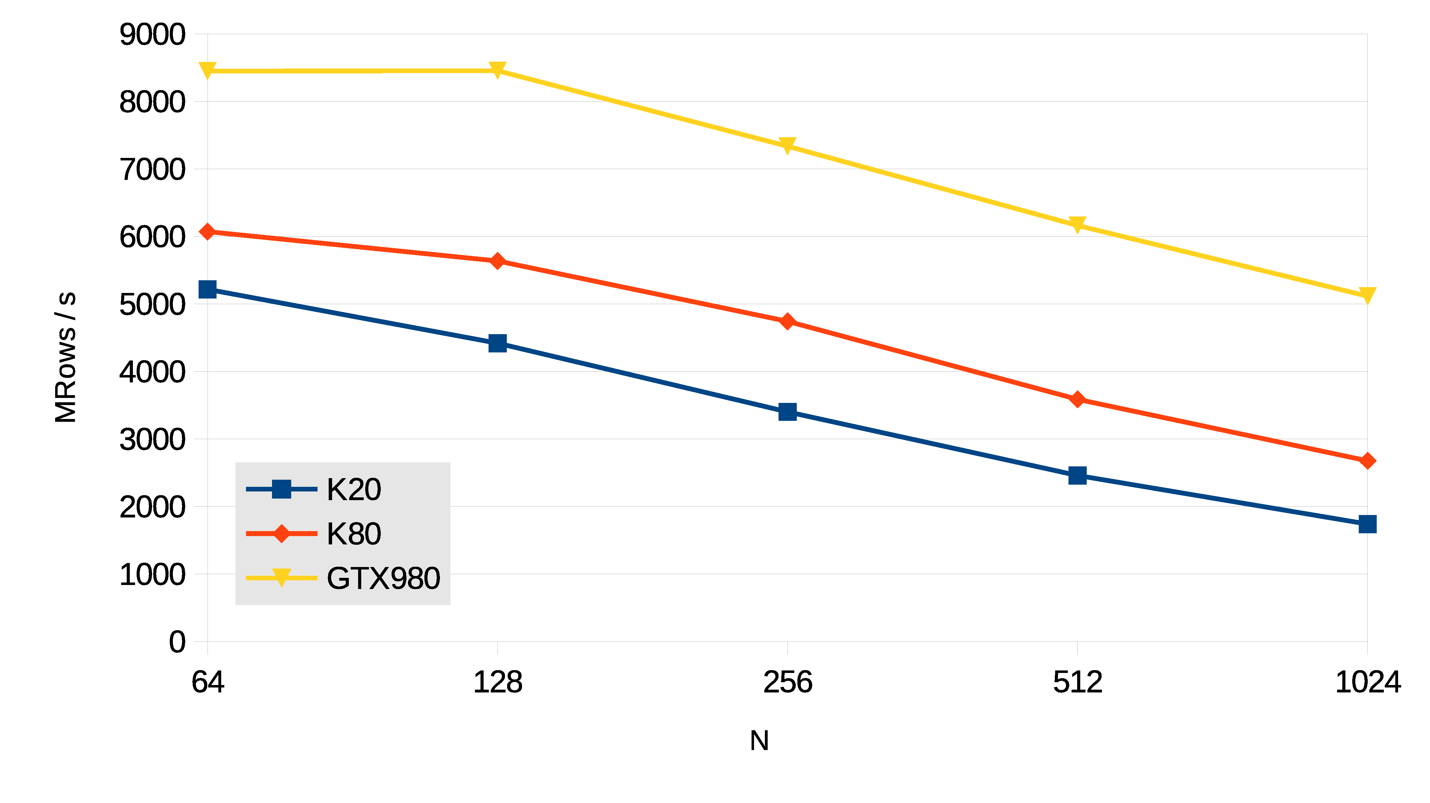
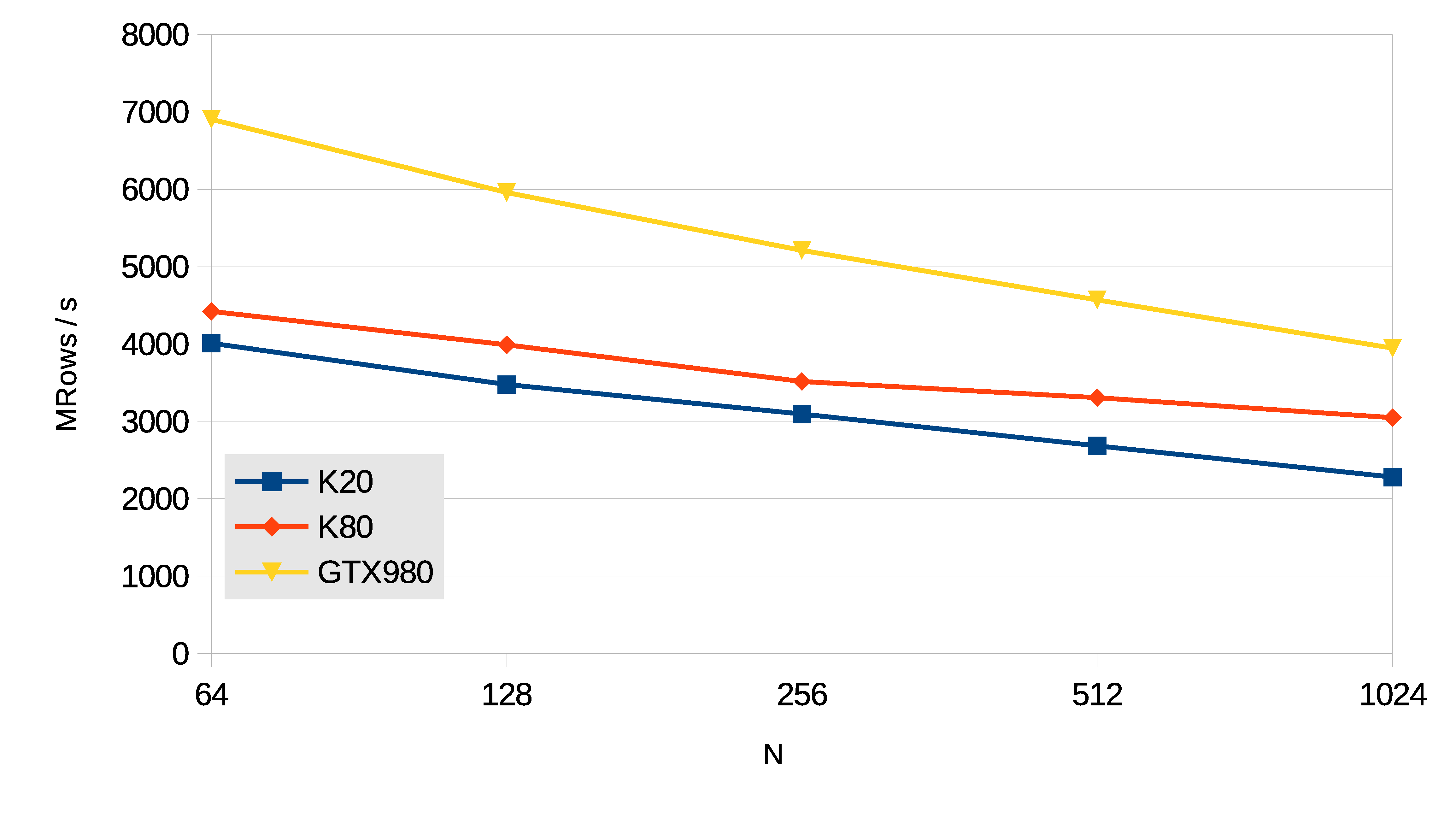
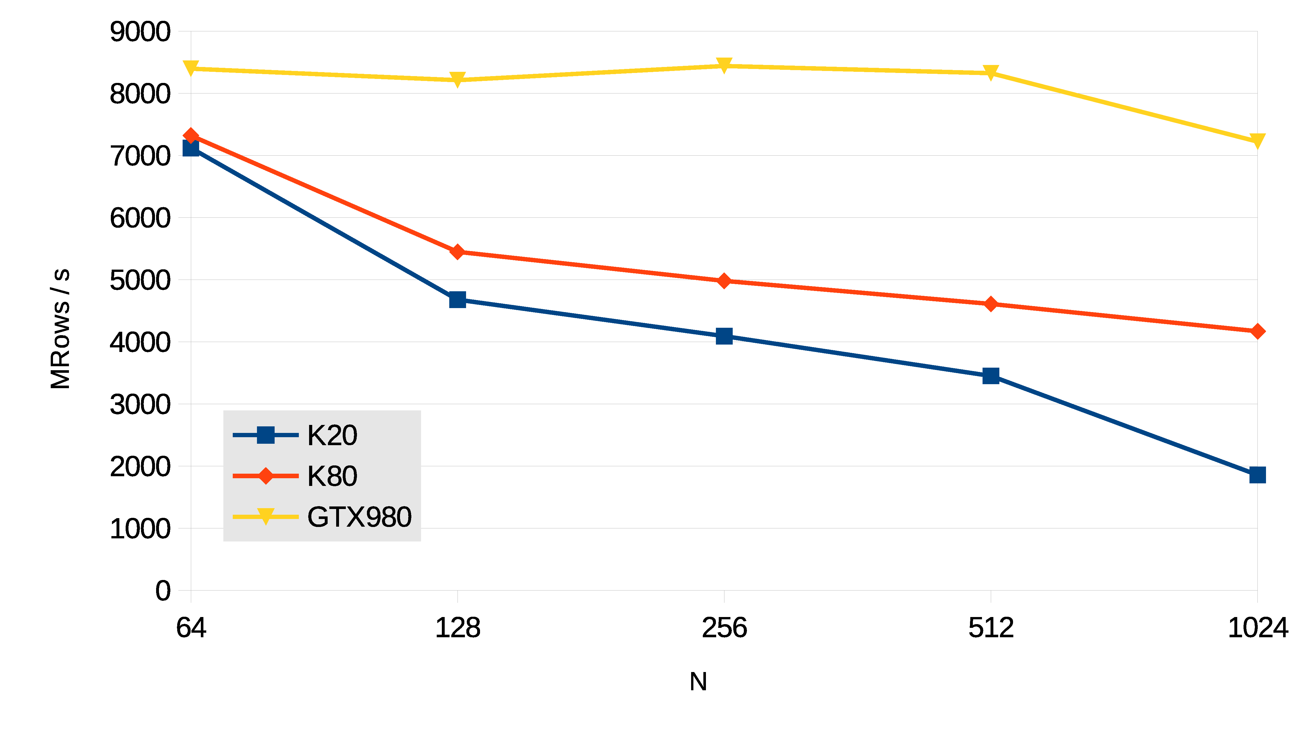
Wang&Mou Tridiagonal Systems

The resolution of tridiagonal equation systems is used in many scientific computing applications, like fluid simulation or the Alternating Direction Implicit method for heat conduction and diffusion equations. The performance of the tridiagonal solver is measured in million rows per second, using the formula:

MRows / s = N · b · 10^-6 / t

In this case N is the number of single-precision equations per tridiagonal system.

As in previous example, tests were ran in single precision using problem sizes in the range N = { 4, ... , 4096 } . Batch execution is employed to compute 2²⁴ / N different problems, thus, as problem size increases the number of batch executions decreases. All the data resides on the GPU memory at the beginning of each test, so there are no data transfers to CPU during the benchmarks.

Three different GPUs with different architectures were used in the current tests:

•   Tesla K20		Kepler architecture
•   Tesla K80		Kepler architecture
•   GeForce GTX980		Maxwell architecture

Cyclic Reduction - Tridiagonal Systems

The performance of the tridiagonal solver is measured in million rows per second, using the formula:

MRows = N · b · 10^-6 / t

In this case N is the number of single-precision equations per tridiagonal system.

Parallel Cyclic Reduction - Tridiagonal Systems

Ladner&Fischer Pattern - Tridiagonal Systems

Ladner&Fischer - Scan

The performance of the scan solver is measured in million elements per second, using the formula:

MData / s = N · b · 10^-6 / t

In this case N is the number of single-precision equations per tridiagonal system.

Kogge&Stone - Scan